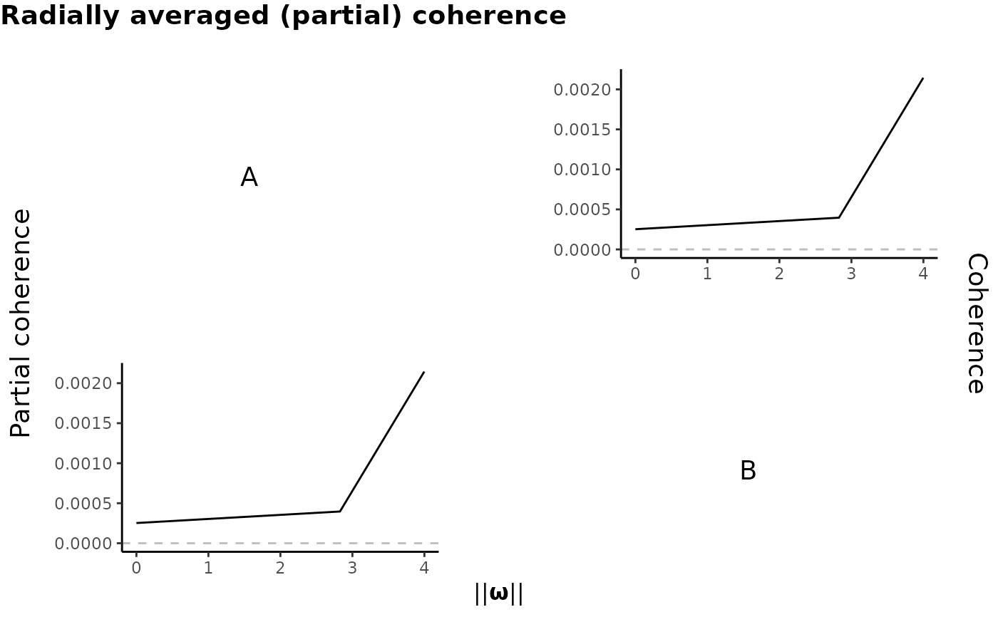
Use ggplot2 package to visualize the coherence and partial coherence.
Arguments
- sp.est
List. The kernel spectral density estimate from
periodogram_smooth().- coh.mat
Coherence matrix from
coherence()withtype = "normal".- partial.coh.mat
Partial coherence matrix from
coherence()withtype = "partial".- xnorm
Logical. If
TRUE(default), plot the radial averaged values. IfFALSE, plot the raw coherence and partial coherence values via heatmap.- ylim
A numeric vector
c(lower, upper)to specify the range to draw for the radially-averaged plot. Not required ifxnorm = FALSE.
Examples
library(spatstat)
lam <- function(x, y, m) {(x^2 + y) * ifelse(m == "A", 2, 1)}
set.seed(227823)
spp <- rmpoispp(lambda = lam, win = square(5), types = c("A","B"))

KSDE.list <- periodogram_smooth(spp, inten.formula = "~ x + y", bandwidth = 1.15)
coh.partial <- coherence(KSDE.list, spp)
#> Number of frequencies to pick the maximum partial coherence: 9 (this value should not be too small).
coh <- coherence(KSDE.list, spp, type = "normal")
#> Number of frequencies to pick the maximum coherence: 9 (this value should not be too small).
plot_coher(KSDE.list, coh, coh.partial)